
Both front end and assembly test and packaging semiconductor factories deploy global dispatching rules alongside local dispatching rules and schedulers to improve productivity. Typically, the global rule ensures the due dates are met and bottleneck tools utilization is optimized by deploying line balance algorithms. These line balance algorithms have different parameters which need to be adjusted based on factory state for a given product mix. Today, these parameters are tuned manually, or in some cases, simulation modeling capabilities are used. It’s difficult to compute the impact of these parameters for all the equipment and all products and process steps in a factory. Manually adjusting the parameters, therefore, could result in negative impact to factory KPIs, and it could take too much time to find an optimal set of parameters using simulation. This use case provides insight into how we tuned the dispatching rule parameters automatically and in significantly less time using SmartFactory Productivity AI.
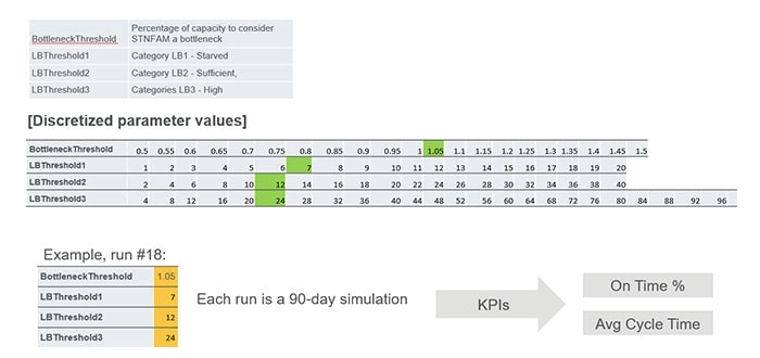
Consider the example shown in figure 1, below. Per the global rule, there are four parameters for determining the bottleneck tool and the line balance thresholds to conclude if the tools are starved, sufficient or high, based on numbers of hours work in process (WIP). The tables show the possible range of values these parameters can take. One option for finding the optimal values of these parameters for a given factory state is to run a simulation model. With each simulation, we choose a different combination of parameter values and measure the resulting KPIs, an approach referred to as grid search in literature. Each run is a 90-day simulation and, for a simulation model to run for 90 days and measure KPIs for on time delivery percentage and cycle time, it will take days. This won’t be practical to use in day-to-day operations.
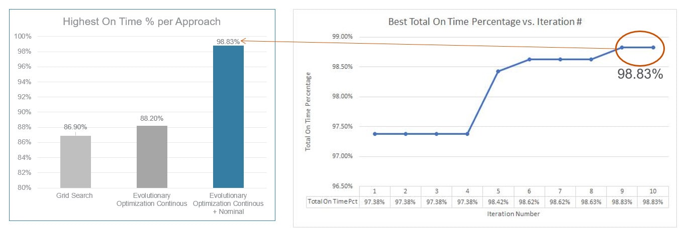
Using this approach, we were able to find the optimal parameter value in hours as compared to days. In each iteration we vary both the line balance parameter values and the combination of bottleneck station families. Where previously it took 300 iterations of grid search to find the best on time percentage of 86.90%, we were able to reach the on-time percentage of 98.83% after just 10 iterations of the model run, as shown in figure 3.
Once the optimal settings are obtained, these can be integrated with existing dispatching rules and scheduling applications and the results can be integrated and recomputed in daily factory operations, as shown in figure 5.
Running for the local KPI of total moves on bottleneck equipment, it took only four iterations to find the optimal bottleneck threshold and line balance thresholds to achieve 20,181 moves.
Simulation optimization is the first step in automating the dispatching and scheduling parameters; further improvements are planned to automate these parameters using reinforcement learning methods.
This use case provides insight into how we tuned the dispatching rule parameters automatically and in significantly less time using SmartFactory AI™ Productivity.
Types of dispatching rules
Dispatching rules are implemented factory wide, typically as global and local rules. The global rule includes line balance logic that enables managing customer commits, and local rules that contain additional logic to optimize the throughput for a given area—like Litho. Both front end and assembly test and packaging semiconductor factories deploy global dispatching rules alongside local dispatching rules and schedulers to improve productivity.
Using algorithms to optimize KPIs
Typically, the global rule ensures the due dates are met and bottleneck tools utilization is optimized by deploying line balance algorithms. These line balance algorithms have different parameters which need to be adjusted based on factory state for a given product mix.
Today, the line balance algorithm parameters are tuned manually, or in some cases, simulation modeling capabilities are used. It’s difficult to compute the impact of these parameters for all the equipment and all products and process steps in a factory. Manually adjusting the parameters, therefore, could result in negative impact to factory KPIs, and it could take too much time to find an optimal set of parameters using simulation.
Limitations of manual tuning
Consider the example shown in figure 1, below. Per the global rule, there are four parameters for determining the bottleneck tool and the line balance thresholds to conclude if the tools are starved, sufficient or high, based on numbers of hours work in process (WIP).
The tables show the possible range of values these parameters can take. One option for finding the optimal values of these parameters for a given factory state is to run a simulation model. With each simulation, we choose a different combination of parameter values and measure the resulting KPIs, an approach referred to as grid search in literature. Each run is a 90-day simulation and, for a simulation model to run for 90 days and measure KPIs for on time delivery percentage and cycle time, it will take days. This won’t be practical to use in day-to-day operations.
Deploying our AI solution
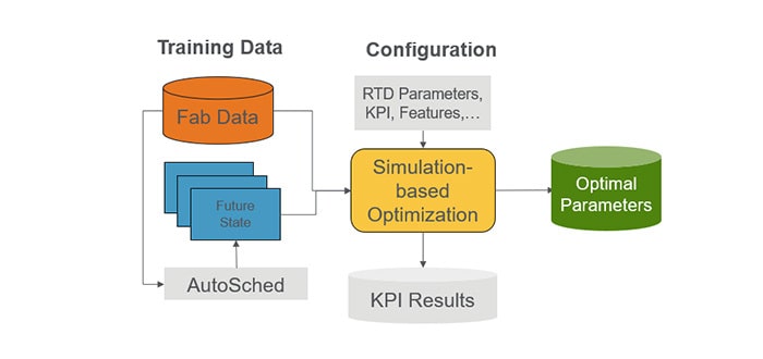
To address this issue, we deployed SmartFactory AI™ Productivity and Evolutionary Optimization combined with Simulated Annealing method to find the optimal parameters for on time delivery and cycle time simultaneously.
Figure 2 shows how this algorithm was deployed using SmartFactory AI™ Productivity, which includes the Simulation AutoSched™ and Fusion modules along with RTD and Activity Manager™.
Fast identification of best on-time percentage
Using this approach, we were able to find the optimal parameter value in hours as compared to days. In each iteration we vary both the line balance parameter values and the combination of bottleneck station families. Where previously it took 300 iterations of grid search to find the best on time percentage of 86.90%, we were able to reach the on-time percentage of 98.83% after just 10 iterations of the model run, as shown in figure 3.
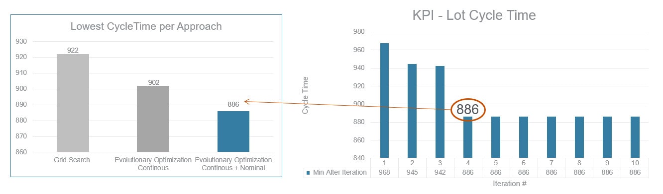
Modeling for cycle time
Applying results to daily operations
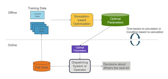
Once the optimal settings are obtained, these can be integrated with existing dispatching rules and scheduling applications and the results can be integrated and recomputed in daily factory operations, as shown in figure 5.
Bottleneck and line balance thresholds
Running for the local KPI of total moves on bottleneck equipment, it took only four iterations to find the optimal bottleneck threshold and line balance thresholds to achieve 20,181 moves.
Conclusion
Simulations allow manufacturers to run multiple combinations of parameter values and measure the resulting KPIs without interfering with production. However, finding optimal values can still be time consuming and not suited to daily operations. Deploying SmartFactory AI™ Productivity and Evolutionary Optimization combined with Simulated Annealing method makes it possible to find optimal settings in a timeframe more realistic for daily operations.
Simulation optimization is the first step in automating the dispatching and scheduling parameters; further improvements are planned to automate these parameters using reinforcement learning methods.
FAQs
What is dispatching in a semiconductor fab?
Dispatching refers to the sequence of lots to process at specific equipment in real-time.
What is the advantage of using dispatching rules?
Dispatching rules can quickly find solutions and prioritize lots to send to tools to optimize productivity.